A convincing image can still contain measurements that are unsuitable for a particular task. Quality control asks whether the inputs, transformations, and outputs meet the requirements of the intended application. This perspective follows evidence through the workflow, from acquisition metadata and reference observations to the final interpretation. It encourages teams to define acceptance conditions before seeing the result, rather than adjusting them to favour a preferred conclusion. The purpose is a repeatable way to distinguish usable observations, observations requiring qualification, and observations that should be excluded from a decision.
This working guide considers spectral band alignment and common grids across peatland forest landscapes. The immediate decision is to select locations for hydrological field review. Useful reference evidence includes water-level records, land-cover observations and dated site visits. The case is an illustrative planning context, with assumptions to check against the actual sensor, landscape and project requirements.
The setting: Peatland forest landscapes
A peatland forest landscape connects vegetation, water conditions, drainage features and land-management history. A satellite image can reveal patterns relevant to these relationships, but a canopy response does not directly measure the depth or condition of the peat below it. Define the monitoring objective carefully. Mapping cover change, identifying areas for hydrological inspection and evaluating a carbon-related parameter require different observations and should not be presented as a single interchangeable result.
A landscape inventory should distinguish forest, open peat, managed land, canals and other surface types that contribute to an observation. Seasonal water conditions and the timing of management events may affect the image record. Optical observations can be limited by cloud and haze, while complementary measurements require their own interpretation. Track usable acquisitions and preserve uncertainty about the timing of a change when it falls within a gap between observations.
Field validation should retain water-level measurements and canopy or land-cover observations as separate evidence streams. Record the date, location and spatial setting of each sample, including its relationship to drainage infrastructure where relevant. A vegetation pattern may help focus a visit without establishing the cause of a hydrological change. More specific claims about emissions, peat condition or restoration performance need suitable measurements and an evaluation method that addresses those variables directly rather than inferring them from greenness alone.
A multiband value should refer to the same ground
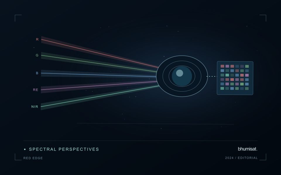
A multispectral analysis combines information from several channels, so their geographic relationship matters. If the channels are displaced, a calculation near a field boundary may combine vegetation in one band with a path, ditch or neighbouring surface in another. The resulting pattern can look like a meaningful spectral difference even though it is partly an alignment artefact. A workflow should therefore consider band alignment before producing indices, classifications or crop parameter estimates, particularly when the target landscape contains small fields and sharp transitions.
Alignment is not the same as assigning every band the same pixel dimensions. Bands may have different native sampling and observation characteristics. Resampling them onto one grid creates a shared representation, but it does not make all channels contain the same original spatial detail. The selected interpolation method can change values around edges and influence derived statistics. Record the target grid, coordinate reference system, pixel alignment and resampling choices so that another analyst can reproduce the combination and evaluate its consequences.
Assess the effects of resampling
Check alignment using features that can be recognised reliably in the relevant channels and are stable at the time of acquisition. Inspect several parts of the area rather than relying on one visually convenient location. A displacement may vary across the image or become more obvious in particular terrain. Quantitative checks should use suitable independent references and report the scale of the remaining error. A correction that appears convincing on a broad overview still needs examination at the spatial scale used by the application.
When evaluating an agricultural model, test whether alignment sensitivity changes its result. For example, compare field statistics with and without a documented interior boundary exclusion, or examine the effects of a small plausible displacement. Such checks help reveal whether a conclusion depends mainly on edge pixels. Avoid using repeated interpolation steps where one controlled transformation would suffice. A clear geometric processing chain makes spectral combinations more defensible and helps ensure that a reported crop difference reflects observations of comparable ground rather than a hidden mismatch between image channels.
Maintain the geographic units of analysis
Many observation services summarise measurements within a field, management block, catchment, forest unit, or other mapped boundary. The meaning of that summary depends on whether the boundary accurately represents the unit being discussed. Start with a clear source for the geometry and record its date, coordinate reference, and intended use. A boundary drawn for visual orientation may require additional checking before it becomes a measurement unit.
Inspect overlaps, gaps, narrow fragments, and features that may have changed since mapping. A geometrically valid polygon can still describe an outdated operational unit. Ask the responsible team how divisions, mergers, new infrastructure, and management changes are recorded. Where pixels or reference measurements cross a boundary, define how they are assigned or excluded so that results remain comparable between analysts and processing runs.
Version the boundaries alongside the observations. If a unit changes, preserve a relationship between the previous and revised geometry rather than replacing the history without explanation. Comparisons through time should identify whether they use a constant spatial unit or the operational units valid at each date. This makes it easier to distinguish a change in the measured surface from a change introduced by the geography used to summarise it.
Match the timing of reference observations
The value of a reference measurement depends partly on how well its timing matches the observation being evaluated. A surface, crop, water body, or instrument state may change between the two measurements. Start by documenting the acquisition time of every source and the period over which the reference observation applies. Avoid treating a date entered during data upload as though it were necessarily the time when the measurement was collected.
Define an acceptable timing relationship for the application. A slowly changing structural feature may tolerate a broader comparison window than a rapidly changing surface condition. The window should be justified by the process being studied and by any available contextual records. If conditions change within that period, consider separating the observations into suitable groups rather than combining them under a single assumption of comparability.
Preserve information about interventions and events between observations. A management operation, rainfall episode, disturbance, or change in sensor configuration can alter the interpretation of a comparison. Record the event and decide whether the pair remains suitable for evaluation. Where the timing mismatch cannot be resolved, describe the comparison as qualified evidence. This is more informative than allowing an uncertain match to influence a performance statistic without explanation.
Bring the evidence back to the decision
Quality control is most useful when its results travel with the information being delivered. Preserve the reasons for accepting or rejecting an observation, and expose limitations that could change the user's interpretation. Review recurring failures as clues about the design of the workflow. A clear quality record supports consistent comparisons between operators and processing versions, while helping the team decide whether a problem originates in acquisition, preparation, interpretation, or the underlying observation requirements.
Sources & further reading
Explore the bhumisat spacecraft concept and our vision towards 2030, or return to the journal.